Getting Started
This section will guide you through the steps required to install the library and provide a simple example to help you get started.
Installation
To use the Bond Graph Toolkit, you need to have Julia installed on your system. If you haven't installed Julia yet, follow the official Julia documentation for instructions specific to your operating system or go directly to the Julia Download page.
Once Julia is installed, you can proceed with installing the Bond Graph toolkit by following these steps:
- Launch Julia by opening the Julia REPL or the Julia command-line interface.
- Enter the package manager by pressing the
]key. You should see the prompt change topkg>. - Inside the package manager, type the following command to add the library:
pkg> add BondGraphToolkit.jl - Wait for Julia to download and install the library and its dependencies. This process may take a few moments depending on your internet connection and system performance.
- Once the installation is complete, you can exit the package manager by pressing the
backspacekey or by typingCtrl+C.
Congratulations! You have successfully installed the library and are ready to start using it.
TODO: add instalation latest version
Quick Example
The source files for all examples can be found in /examples.
Let's explore the capabilities of the library through a quick example of modeling a basic dynamic system, an RC circuit. The RC circuit is a fundamental electrical circuit consisting of a resistor (R) and a capacitor (C), as depicted in the figure below:
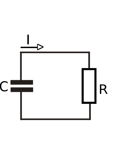
By using the Kirchhoff's law we have the following linear differential equation that describes the charge on the capacitor along the time.
\[C \frac{dV}{dt} + \frac{V}{R} = 0\]
To model the RC circuit using the bond graph method, we can connect the compliance (C) and resistance (R) elements to a zero-junction, as shown in the bond graph diagram:

Bond Graph Toolkit
We can use the Bond Graph Toolkit to model and get the RC circuit equations and then solve the system, as presented in the code below.
# Import the required libraries
using BondGraph
using DifferentialEquations
using Plots

# Define the elements of the RC circuit
@named C = Spring(k=1 / 1.0)   # Electric capacitance (F)
@named R = Damper(c=1.0)       # Electric resistance (Ohm)

# Create the RC circuit model by connecting the elements
@named model = Junction0(R, C)
# Simplify the system equations
@named sys = simplifysys(model)

# Set the time span for simulation
tspan = (0, 10)
# Define the initial conditions
initial_conditions = [R.power.f => 0.0, C.q => 1.0]

# Define the ODE problem
prob = ODEProblem(sys, initial_conditions, tspan)
# Solve the ODE problem
sol = solve(prob)
# Plot the results
plot(sol, xlabel="Time", ylabel="Amplitude")
Moreover, we can generate the bond graph diagram of the model using the generate_graph function.
generate_graph(model)Print the system states
states(sys)1-element Vector{SymbolicUtils.BasicSymbolic{Real}}:
C₊q(t)Print the system parameters
parameters(sys)2-element Vector{SymbolicUtils.BasicSymbolic{Real}}:
C₊C
R₊RPrint the simplified equations of the system
equations(sys)\[ \begin{align} \frac{\mathrm{d} C_{+}q\left( t \right)}{\mathrm{d}t} =& \frac{ - C_{+}q\left( t \right)}{C_{+}C R_{+}R} \end{align} \]
In the code snippets, we start by importing the libraries BondGraph, DifferentialEquations, and Plots. Then, ee define the elements of the RC circuit, namely the compliance C and the resistance R, using the functions Spring and Damper from the BondGraphToolkit package.
Next, we create the RC circuit model by connecting the elements R and C to a zero-junction using the Junction0 function. We use the simplifysys function to obtain a more concise representation of the system, which is stored in the variable sys.
To simulate the system, We first define the time span for the simulation using the tuple (0, 10). Then, we specify the initial conditions of the system in the initial_conditions dictionary, where we set the initial charge on the capacitor C to $1.0$ and the initial flow through the resistor R to $0.0$.
Using the ODEProblem function from DifferentialEquations, we define the ODE problem to be solved by passing the system sys, the initial conditions, and the time span. We solve the ODE problem using the solve function.
Finally, we visualize the results by plotting the solution (sol) using the plot function from Plots. The x-axis represents time, and the y-axis represents the amplitude of the variables in the system.
This section was generated using Literate.jl.