DC Motor
The source files for all examples can be found in /examples.
The DC motor is a commonly used actuator that provides rotary motion to a mechanical system. It converts electrical energy into rotational mechanical energy. Thus, modeling it with a bond graph requires an additional port to the zero and one junctions. The system can be represented as an equivalent circuit of the armature and the free-body diagram of the rotor illustrated below:
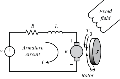
DC Motor model
We assumed that the rotor and shaft are rigid to model the DC motor coupled with a shaft. We also considered the shaft friction proportional to its angular velocity, representing a viscous friction model.
The torque generated by a DC motor is typically proportional to the armature current ($i$) and the strength of the magnetic field. However, we will assume a constant magnetic field for simplicity, resulting in the motor torque being proportional to the armature current. We represent this relationship using a constant factor $k_\tau$, which gives us the following equation:
\[\tau = k_\tau i\]
The back electromotive force generated by the motor torque is proportional to the angular velocity of the shaft ($\dot{\theta}$) through a constant factor $k_e$:
\[e = k_e \dot{\theta}\]
The motor torque constant ($k_\tau$) and the back electromotive force ($k_e$) are equal, denoted as $k$.
Finally, based on Newton's 2nd law and Kirchhoff's voltage law, we can derive the following governing equations for the system:
\[J\ddot{\theta} + c\,\dot{\theta} = k\,i ,\]
\[L\frac{di}{dt} + R\,i = V - k\,\dot{\theta},\]
where $J$ represents the moment of inertia of the rotor, $c$ is the viscous friction coefficient, $L$ and $R$ are the armature inductance and resistance, respectively. By solving these equations, we can analyze the dynamic behavior of the DC motor and shaft system.
See also DC Motor Speed: System Modeling
Bond Graph Model
To model the DC motor depicted in the figure above, we can use the bond graph approach and represent the system with the following bond graph:
TODO: update the bond graph 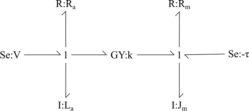
In this representation, the inertance elements (I) correspond to the moment of inertia of the rotor ($J$) in the mechanical domain and the armature inductance ($L$) in the electrical domain. The resistance elements (R) represent the viscous friction coefficient ($c$) in the mechanical domain and the armature electrical resistance ($R_a$).
The gyrator (GY) port describes the electrical current and torque relationship, with the constant $k$ representing its value.
Bond-graph toolkit
In this example we are going to first build and simulate the bond graph model for the DC motor. Then we are going to use the DC motor differential equations obtained based Newton's 2nd law and Kirchhoff's voltage law to compare the results.
Firstly, we need to import the bond-graph toolkit module to model the system and the DifferentialEquations.jl to solve the resultant ODE. Also, we import the independent variable t from the bond-graph toolkit to define a custom forcing term.
using BondGraph
using BondGraph: t, D
using DifferentialEquations
using ModelingToolkit
using Plots
using Symbolics.Latexify
Building the model
Before defining a system, we need to define the single port elements of the system. Then, we define the electrical inductance (L), resitance (R) and the source of effort (V, voltage applied), elements as follows:
@named L = Mass(m=0.5)        # (H) Electric inductance
@named R = Damper(c = 1.0)    # (Ohm) Electric resistance
@named V = Se(12.0)           # (V) Voltage
\[ \begin{align} power_{+}e\left( t \right) =& 12 \end{align} \]
For the mechanical part we define the shaft moment of inertia (J), viscous friction (c) and the source of effort (τ) as follows:
@named J = Mass(m = 0.01)     # (kg⋅m^2) Shaft moment of inertia
@named c = Damper(c = 0.1)    # (N⋅m⋅s) Shaft viscous friction
@named τ = Se(1.0)            # (N⋅m) Applied torque on the shaft
\[ \begin{align} power_{+}e\left( t \right) =& 1 \end{align} \]
Finally the current-torque constant is defined as:
g = 0.01 # DC motor torque constant0.01We build the system by simply passing the one-port elements to the 1-junction function as arguments for the mechanical and electrical part, respectively.
@named jm = Junction1(τ, [-1, c], [-1, J])    # Mechanical part
@named je = Junction1(V, [-1, R], [-1, L])    # Electical part
\[ \begin{equation} \left[ \begin{array}{c} \mathrm{connect}\left( V_{+}power, power \right) \\ \mathrm{connect}\left( power, R_{+}power \right) \\ \mathrm{connect}\left( power, L_{+}power \right) \\ V_{+}power_{+}e\left( t \right) = 12 \\ R_{+}power_{+}e\left( t \right) = R_{+}R R_{+}power_{+}f\left( t \right) \\ \frac{\mathrm{d} L_{+}power_{+}f\left( t \right)}{\mathrm{d}t} = \frac{L_{+}power_{+}e\left( t \right)}{L_{+}I} \\ \end{array} \right] \end{equation} \]
Then, we couple mechanical and electrical domains using the gyrator port.
eqs = []
@named gy = mGY(je, jm, g = g, coneqs = eqs)

### Build the system
\[ \begin{align} pout_{+}e\left( t \right) =& - 0.01 pin_{+}f\left( t \right) \\ pin_{+}e\left( t \right) =& 0.01 pout_{+}f\left( t \right) \end{align} \]
We build the system by first creating a ODESystem with mGY generated equations and setting the independent variable as t.
@named mdl = ODESystem(eqs, t)\[ \begin{equation} \left[ \begin{array}{c} \mathrm{connect}\left( je_{+}power, gy_{+}pin \right) \\ \mathrm{connect}\left( gy_{+}pout, jm_{+}power \right) \\ \end{array} \right] \end{equation} \]
Then, we need to add the subsystems to the model.
mdl = compose(mdl, gy, je, jm)\[ \begin{equation} \left[ \begin{array}{c} \mathrm{connect}\left( je_{+}power, gy_{+}pin \right) \\ \mathrm{connect}\left( gy_{+}pout, jm_{+}power \right) \\ gy_{+}pout_{+}e\left( t \right) = - 0.01 gy_{+}pin_{+}f\left( t \right) \\ gy_{+}pin_{+}e\left( t \right) = 0.01 gy_{+}pout_{+}f\left( t \right) \\ \mathrm{connect}\left( V_{+}power, power \right) \\ \mathrm{connect}\left( power, R_{+}power \right) \\ \mathrm{connect}\left( power, L_{+}power \right) \\ je_{+}V_{+}power_{+}e\left( t \right) = 12 \\ je_{+}R_{+}power_{+}e\left( t \right) = je_{+}R_{+}R je_{+}R_{+}power_{+}f\left( t \right) \\ \frac{\mathrm{d} je_{+}L_{+}power_{+}f\left( t \right)}{\mathrm{d}t} = \frac{je_{+}L_{+}power_{+}e\left( t \right)}{je_{+}L_{+}I} \\ \mathrm{connect}\left( \tau_{+}power, power \right) \\ \mathrm{connect}\left( power, c_{+}power \right) \\ \mathrm{connect}\left( power, J_{+}power \right) \\ jm_+\tau_{+}power_{+}e\left( t \right) = 1 \\ jm_{+}c_{+}power_{+}e\left( t \right) = jm_{+}c_{+}R jm_{+}c_{+}power_{+}f\left( t \right) \\ \frac{\mathrm{d} jm_{+}J_{+}power_{+}f\left( t \right)}{\mathrm{d}t} = \frac{jm_{+}J_{+}power_{+}e\left( t \right)}{jm_{+}J_{+}I} \\ \end{array} \right] \end{equation} \]
Analysing the model
We can visualize the bond-graph connections by generating a graph plot of the model.
generate_graph(mdl)We can obtain the bond-graph equations using the code below.
equations(expand_connections(mdl))\[ \begin{align} gy_{+}pout_{+}e\left( t \right) =& - 0.01 gy_{+}pin_{+}f\left( t \right) \\ gy_{+}pin_{+}e\left( t \right) =& 0.01 gy_{+}pout_{+}f\left( t \right) \\ je_{+}V_{+}power_{+}e\left( t \right) =& 12 \\ je_{+}R_{+}power_{+}e\left( t \right) =& je_{+}R_{+}R je_{+}R_{+}power_{+}f\left( t \right) \\ \frac{\mathrm{d} je_{+}L_{+}power_{+}f\left( t \right)}{\mathrm{d}t} =& \frac{je_{+}L_{+}power_{+}e\left( t \right)}{je_{+}L_{+}I} \\ jm_+\tau_{+}power_{+}e\left( t \right) =& 1 \\ jm_{+}c_{+}power_{+}e\left( t \right) =& jm_{+}c_{+}R jm_{+}c_{+}power_{+}f\left( t \right) \\ \frac{\mathrm{d} jm_{+}J_{+}power_{+}f\left( t \right)}{\mathrm{d}t} =& \frac{jm_{+}J_{+}power_{+}e\left( t \right)}{jm_{+}J_{+}I} \\ - je_{+}power_{+}f\left( t \right) =& je_{+}V_{+}power_{+}f\left( t \right) \\ - je_{+}power_{+}f\left( t \right) =& - je_{+}L_{+}power_{+}f\left( t \right) \\ - je_{+}power_{+}f\left( t \right) =& - je_{+}R_{+}power_{+}f\left( t \right) \\ 0 =& - gy_{+}pout_{+}e\left( t \right) - jm_{+}J_{+}power_{+}e\left( t \right) - jm_{+}c_{+}power_{+}e\left( t \right) + jm_+\tau_{+}power_{+}e\left( t \right) \\ jm_+\tau_{+}power_{+}f\left( t \right) =& - jm_{+}J_{+}power_{+}f\left( t \right) \\ jm_+\tau_{+}power_{+}f\left( t \right) =& - gy_{+}pout_{+}f\left( t \right) \\ jm_+\tau_{+}power_{+}f\left( t \right) =& - jm_{+}c_{+}power_{+}f\left( t \right) \\ je_{+}power_{+}e\left( t \right) =& gy_{+}pin_{+}e\left( t \right) \\ 0 =& - je_{+}L_{+}power_{+}e\left( t \right) - je_{+}R_{+}power_{+}e\left( t \right) - je_{+}power_{+}e\left( t \right) + je_{+}V_{+}power_{+}e\left( t \right) \\ je_{+}power_{+}f\left( t \right) =& gy_{+}pin_{+}f\left( t \right) \end{align} \]
The equations of the model above were not simplified and represent the bond-graphs equations directly derived from the connections. Then, we simplify the DAE above and obtain the ODE. The simplified set of equations is required for using solve from DifferentialEquations.jl
@named sys = simplifysys(mdl)\[ \begin{align} \frac{\mathrm{d} je_{+}L_{+}power_{+}f\left( t \right)}{\mathrm{d}t} =& \frac{12 - 0.01 jm_{+}J_{+}power_{+}f\left( t \right) - je_{+}R_{+}R je_{+}L_{+}power_{+}f\left( t \right)}{je_{+}L_{+}I} \\ \frac{\mathrm{d} jm_{+}J_{+}power_{+}f\left( t \right)}{\mathrm{d}t} =& \frac{1 + 0.01 je_{+}L_{+}power_{+}f\left( t \right) - jm_{+}c_{+}R jm_{+}J_{+}power_{+}f\left( t \right)}{jm_{+}J_{+}I} \end{align} \]
Print system states
states(sys)2-element Vector{SymbolicUtils.BasicSymbolic{Real}}:
je₊L₊power₊f(t)
jm₊J₊power₊f(t)Print system parameters
parameters(sys)4-element Vector{SymbolicUtils.BasicSymbolic{Real}}:
je₊L₊I
je₊R₊R
jm₊c₊R
jm₊J₊IPrint the system simplified equations
equations(sys)\[ \begin{align} \frac{\mathrm{d} je_{+}L_{+}power_{+}f\left( t \right)}{\mathrm{d}t} =& \frac{12 - 0.01 jm_{+}J_{+}power_{+}f\left( t \right) - je_{+}R_{+}R je_{+}L_{+}power_{+}f\left( t \right)}{je_{+}L_{+}I} \\ \frac{\mathrm{d} jm_{+}J_{+}power_{+}f\left( t \right)}{\mathrm{d}t} =& \frac{1 + 0.01 je_{+}L_{+}power_{+}f\left( t \right) - jm_{+}c_{+}R jm_{+}J_{+}power_{+}f\left( t \right)}{jm_{+}J_{+}I} \end{align} \]
By comparison, we can see that the equations above are the same as the canonical form of the harmonic oscillator presented at the beginning.
We can generate LaTeX code from the equations
latexify(equations(sys))\begin{align} \frac{\mathrm{d} je{+}L{+}power{+}f\left( t \right)}{\mathrm{d}t} =& \frac{12 - 0.01 jm{+}J{+}power{+}f\left( t \right) - je{+}R{+}R je{+}L{+}power{+}f\left( t \right)}{je{+}L{+}I} \ \frac{\mathrm{d} jm{+}J{+}power{+}f\left( t \right)}{\mathrm{d}t} =& \frac{1 + 0.01 je{+}L{+}power{+}f\left( t \right) - jm{+}c{+}R jm{+}J{+}power{+}f\left( t \right)}{jm{+}J{+}I} \end{align}
Simulate the system
Bond graph model
Define the simulation time
tspan = (0, 10)(0, 10)Generate an ODEProblem as in the ModelingToolkit, passing the simulation interval.
prob = ODEProblem(sys, [], tspan)ODEProblem with uType Vector{Float64} and tType Int64. In-place: true
timespan: (0, 10)
u0: 2-element Vector{Float64}:
0.0
0.0Use the solve to simulate the system.
sol = solve(prob)
plot(sol, xlabel = "Time", ylabel = "Amplitude")
DC motor model
First, we define the state variables of the DC motor system, which are the $i$, $\theta$, and $\cdot{\theta}$. They represent the armature current, shaft angle, and shaft angular velocity, respectively.
@variables i(t) = 0.0           # Armature current
@variables θ(t) = 0.0           # Shaft angle
@variables θ̇(t) = 0.0           # Shaft angular velocity
\[ \begin{equation} \left[ \begin{array}{c} θ̇\left( t \right) \\ \end{array} \right] \end{equation} \]
Then, we define the DC motor system parameters.
Lᵥ = 0.5                      # (H) - Inductance
Rᵥ = 1.0                      # (Ohm) - Resistance
Uᵥ = 12.0                     # (V) - Voltage

Jᵥ = 0.01                     # (kg*m²) - Moment of inertia of the rotor
bᵥ = 0.1                      # (N*m*s) - Motor viscous friction constant
Tᵥ = 1.0 # (N*m) - Motor torque1.0Define the differential equations that represent the governing equations of the system. They include the equation for shaft angular acceleration, armature current, and the derivative of the shaft angle.
eqs_t = [
    Jᵥ * D(θ̇) ~ Tᵥ + g * i - bᵥ * θ̇,   # Equation for shaft angular acceleration
    Lᵥ * D(i) ~ -Rᵥ * i + Uᵥ - g * θ̇,   # Equation for armature current
    D(θ) ~ θ̇                          # Equation for shaft angle derivative
]
\[ \begin{align} 0.01 \frac{\mathrm{d} θ̇\left( t \right)}{\mathrm{d}t} =& 1 + 0.01 i\left( t \right) - 0.1 θ̇\left( t \right) \\ 0.5 \frac{\mathrm{d} i\left( t \right)}{\mathrm{d}t} =& 12 - 0.01 θ̇\left( t \right) - i\left( t \right) \\ \frac{\mathrm{d} \theta\left( t \right)}{\mathrm{d}t} =& θ̇\left( t \right) \end{align} \]
Then, we use the equations defined above to create the ODESystem.
@named sys_t = ODESystem(eqs_t, t)\[ \begin{align} \frac{\mathrm{d} \theta\left( t \right)}{\mathrm{d}t} =& θ̇\left( t \right) \\ 0.01 \frac{\mathrm{d} θ̇\left( t \right)}{\mathrm{d}t} =& 1 + 0.01 i\left( t \right) - 0.1 θ̇\left( t \right) \\ 0.5 \frac{\mathrm{d} i\left( t \right)}{\mathrm{d}t} =& 12 - 0.01 θ̇\left( t \right) - i\left( t \right) \end{align} \]
We simplify the ODE using the structural_simplify function of the ModelingToolkit.jl library. This procedure is required for using solve from DifferentialEquations.jl
sys_t = structural_simplify(sys_t)\[ \begin{align} \frac{\mathrm{d} \theta\left( t \right)}{\mathrm{d}t} =& θ̇\left( t \right) \\ \frac{\mathrm{d} θ̇\left( t \right)}{\mathrm{d}t} =& - 100 \left( -1 - 0.01 i\left( t \right) + 0.1 θ̇\left( t \right) \right) \\ \frac{\mathrm{d} i\left( t \right)}{\mathrm{d}t} =& - 2 \left( -12 + 0.01 θ̇\left( t \right) + i\left( t \right) \right) \end{align} \]
Define the ODEproblem to simulate with the time span defined for the bond graph simulation.
prob_t = ODEProblem(sys_t, [], tspan)ODEProblem with uType Vector{Float64} and tType Int64. In-place: true
timespan: (0, 10)
u0: 3-element Vector{Float64}:
0.0
0.0
0.0Use the solve to simulate the system.
sol_t = solve(prob_t, reltol = 1e-8, abstol = 1e-8);Plot the results
plot(sol_t.t, sol_t[θ̇], label = "Angular Velocity")
plot!(sol_t.t, sol_t[i], label = "Armature Current")
Compare models
We will graphically compare the results obtained from the bond graph representation and the direct simulation of the system using the governing differential equations.
Electrical domain
plot(sol.t, sol[je.L.power.f], label = "Bond-graph", ylabel = "Current (A)")
plot!(sol_t.t, sol_t[i], label = "Model", xlabel = "Time (s)")
Mechanical domain
plot(sol.t, sol[jm.J.power.f], label = "Bond-graph", ylabel = "Angular velocity (rad/s)")
plot!(sol_t.t, sol_t[θ̇], label = "Model", xlabel = "Time (s)")
As we can see, the simulation, based on the bond graph model, replicated the expected dynamics.
This page was generated using Literate.jl.