Harmonic Oscillator

The source files for all examples can be found in /examples.

The harmonic oscillator is a classic example of a dynamic system characterized by oscillatory behavior. In the mechanical domain, it can be represented as a mass-spring-damper system, as illustrated below:

Mass-Spring-Damper System

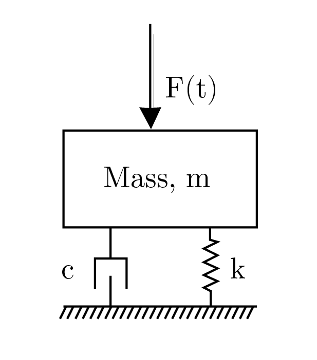
The following differential equation governs the motion of the harmonic oscillator:

\[m\,\frac{d^2 x}{dt^2} + c\,\frac{d^2 x}{dt^2} + k\,x = F(t), $ where $x\]

is the position, $m$ is the mass, $c$ is the damping coefficient, $k$ is the spring stiffness, and $F(t)$ is an external force applied to the system.

To model the harmonic oscillator using the bond graph method, we can connect the inertance (I), compliance (C), and resistance (R) elements to a 1-junction, as depicted in the bond graph diagram:

Bond Graph Representation

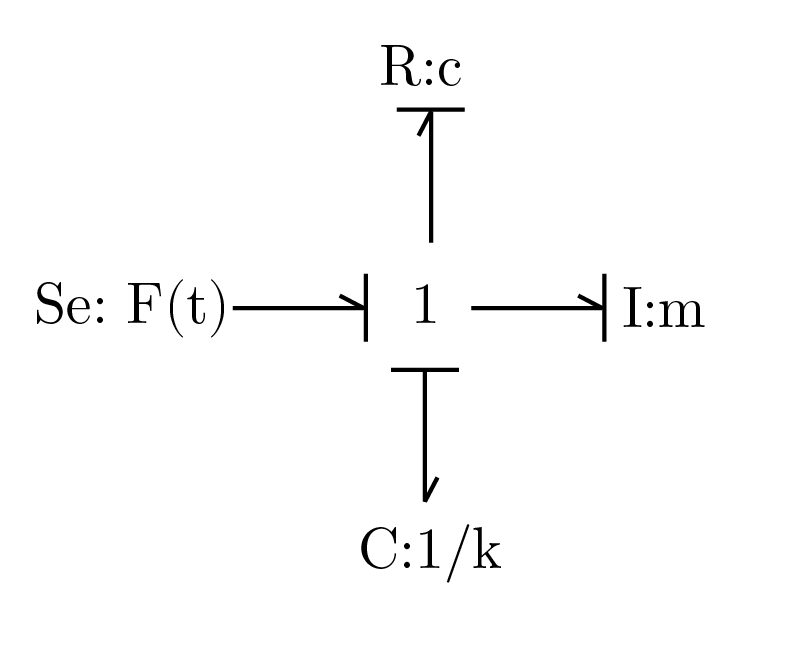
In this representation, the inertance element (I) corresponds to the mass (m) in the mechanical system, the compliance element (C) corresponds to the spring constant (k), and the resistance element (R) represents the damping coefficient (c).

Bond-graph toolkit

Firstly, we need to import the bond-graph toolkit module to model the system and the DifferentialEquations.jl to solve the resultant ODE. Also, we import the independent variable t from the bond-graph toolkit to define a custom forcing term.

using BondGraph
using BondGraph: t, D
using DifferentialEquations
using ModelingToolkit
using Plots
using Symbolics.Latexify

Building the model

Before defining a system, we need to define the single port elements of the system. Then, we define the mass, spring, and damper elements as follows:

@named m = Mass(m = 1.0);      # (kg)
@named s = Spring(k = 1.0);    # (N/m)
@named d = Damper(c = 1.0);    # (N⋅m⋅s)

┌ Warning: power contains 0 flow variables, yet 2 regular (non-flow, non-stream, non-input, non-output) variables. This could lead to imbalanced model that are difficult to debug. Consider marking some of the regular variables as input/output variables.
└ @ ModelingToolkit ~/.julia/packages/ModelingToolkit/GFEA2/src/systems/connectors.jl:40
┌ Warning: power contains 0 flow variables, yet 2 regular (non-flow, non-stream, non-input, non-output) variables. This could lead to imbalanced model that are difficult to debug. Consider marking some of the regular variables as input/output variables.
└ @ ModelingToolkit ~/.julia/packages/ModelingToolkit/GFEA2/src/systems/connectors.jl:40
┌ Warning: power contains 0 flow variables, yet 2 regular (non-flow, non-stream, non-input, non-output) variables. This could lead to imbalanced model that are difficult to debug. Consider marking some of the regular variables as input/output variables.
└ @ ModelingToolkit ~/.julia/packages/ModelingToolkit/GFEA2/src/systems/connectors.jl:40

The forcing term can be set as an expression or even a Julia function. In this example, we will first intialize a generic forcing term that will be defined before solving the ODE.

@parameters F(t)
@named f = Se(F)

\[ \begin{align} power_{+}e\left( t \right) =& F\left( t \right) \end{align} \]

Then, we build the system by simply passing the one-port elements to the 1-junction function as arguments.

@named mdl = Junction1(m, d, s, [-1, f]);

┌ Warning: power contains 0 flow variables, yet 2 regular (non-flow, non-stream, non-input, non-output) variables. This could lead to imbalanced model that are difficult to debug. Consider marking some of the regular variables as input/output variables.
└ @ ModelingToolkit ~/.julia/packages/ModelingToolkit/GFEA2/src/systems/connectors.jl:40

Analysing the model

We can visualize the bond-graph connections by generating a graph plot of the model.

generate_graph(mdl)

We can obtain the bond-graph equations using the code below.

equations(expand_connections(mdl))

\[ \begin{align} \frac{\mathrm{d} m_{+}power_{+}f\left( t \right)}{\mathrm{d}t} =& \frac{m_{+}power_{+}e\left( t \right)}{m_{+}I} \\ d_{+}power_{+}e\left( t \right) =& d_{+}R d_{+}power_{+}f\left( t \right) \\ s_{+}power_{+}e\left( t \right) =& \frac{s_{+}q\left( t \right)}{s_{+}C} \\ \frac{\mathrm{d} s_{+}q\left( t \right)}{\mathrm{d}t} =& s_{+}power_{+}f\left( t \right) \\ f_{+}power_{+}e\left( t \right) =& f_{+}F\left( t \right) \\ s_{+}power_{+}f\left( t \right) =& d_{+}power_{+}f\left( t \right) \\ s_{+}power_{+}f\left( t \right) =& m_{+}power_{+}f\left( t \right) \\ s_{+}power_{+}f\left( t \right) =& - f_{+}power_{+}f\left( t \right) \\ 0 =& - f_{+}power_{+}e\left( t \right) + d_{+}power_{+}e\left( t \right) + m_{+}power_{+}e\left( t \right) + s_{+}power_{+}e\left( t \right) \end{align} \]

The equations of the model above were not simplified and represent the bond-graphs equations directly derived from the connections. Then, we simplify the DAE above and obtain the ODE. The simplified set of equations is required for using solve from DifferentialEquations.jl

@named sys = simplifysys(mdl)

\[ \begin{align} \frac{\mathrm{d} m_{+}power_{+}f\left( t \right)}{\mathrm{d}t} =& \frac{\frac{ - s_{+}q\left( t \right)}{s_{+}C} - d_{+}R m_{+}power_{+}f\left( t \right) + f_{+}F\left( t \right)}{m_{+}I} \\ \frac{\mathrm{d} s_{+}q\left( t \right)}{\mathrm{d}t} =& m_{+}power_{+}f\left( t \right) \end{align} \]

Print system states

states(sys)

2-element Vector{SymbolicUtils.BasicSymbolic{Real}}:
 m₊power₊f(t)
 s₊q(t)

Print system parameters

parameters(sys)

4-element Vector{SymbolicUtils.BasicSymbolic{Real}}:
 d₊R
 f₊F(t)
 m₊I
 s₊C

Print the system simplified equations

equations(sys)

By comparison, we can see that the equations above are the same as the canonical form of the harmonic oscillator presented at the beginning.

We can generate LaTeX code from the equations

latexify(equations(sys))

\begin{align} \frac{\mathrm{d} m{+}power{+}f\left( t \right)}{\mathrm{d}t} =& \frac{\frac{ - s{+}q\left( t \right)}{s{+}C} - d{+}R m{+}power{+}f\left( t \right) + f{+}F\left( t \right)}{m{+}I} \ \frac{\mathrm{d} s{+}q\left( t \right)}{\mathrm{d}t} =& m{+}power{+}f\left( t \right) \end{align}

Simulate the system

Unforced case

Now, we are going to consider only the unforced case. Therefore, $F(t) = 0$. Thus, we update the force function on the system.

sys_unforced = substitute(sys, Dict(f.F => 0.0))

\[ \begin{align} \frac{\mathrm{d} m_{+}power_{+}f\left( t \right)}{\mathrm{d}t} =& \frac{\frac{ - s_{+}q\left( t \right)}{s_{+}C} - d_{+}R m_{+}power_{+}f\left( t \right)}{m_{+}I} \\ \frac{\mathrm{d} s_{+}q\left( t \right)}{\mathrm{d}t} =& m_{+}power_{+}f\left( t \right) \end{align} \]

Define the simulation time

tspan = (0, 10)

(0, 10)

When defining the ODEProblem as in the ModelingToolkit, we can define the initial value of the states.

prob = ODEProblem(sys_unforced, [m.power.f => 0.0, s.q => 1.0], tspan)

ODEProblem with uType Vector{Float64} and tType Int64. In-place: true
timespan: (0, 10)
u0: 2-element Vector{Float64}:
 0.0
 1.0

Use the solve to simulate the system.

sol = solve(prob)
plot(sol, xlabel = "Time", ylabel = "Amplitude")

Forced case

Now, we are going to consider the forced case, where $F(t) = sin(t)$. Thus, we update the force function on the system.

sys_forced = substitute(sys, Dict(f.F => sin(t)))

\[ \begin{align} \frac{\mathrm{d} m_{+}power_{+}f\left( t \right)}{\mathrm{d}t} =& \frac{\frac{ - s_{+}q\left( t \right)}{s_{+}C} - d_{+}R m_{+}power_{+}f\left( t \right) + \sin\left( t \right)}{m_{+}I} \\ \frac{\mathrm{d} s_{+}q\left( t \right)}{\mathrm{d}t} =& m_{+}power_{+}f\left( t \right) \end{align} \]

Define the simulation time

tspan = (0, 10)

(0, 10)

When defining the ODEProblem as in the ModelingToolkit we can define the initial value of the states.

prob = ODEProblem(sys_forced, [m.power.f => 0.0, s.q => 0.0], tspan)

ODEProblem with uType Vector{Float64} and tType Int64. In-place: true
timespan: (0, 10)
u0: 2-element Vector{Float64}:
 0.0
 0.0

Use the solve to simulate the system.

sol = solve(prob)
plot(sol, xlabel = "Time", ylabel = "Amplitude")

This page was generated using Literate.jl.